Hooke's Law and Energy Lab

Physics Overview

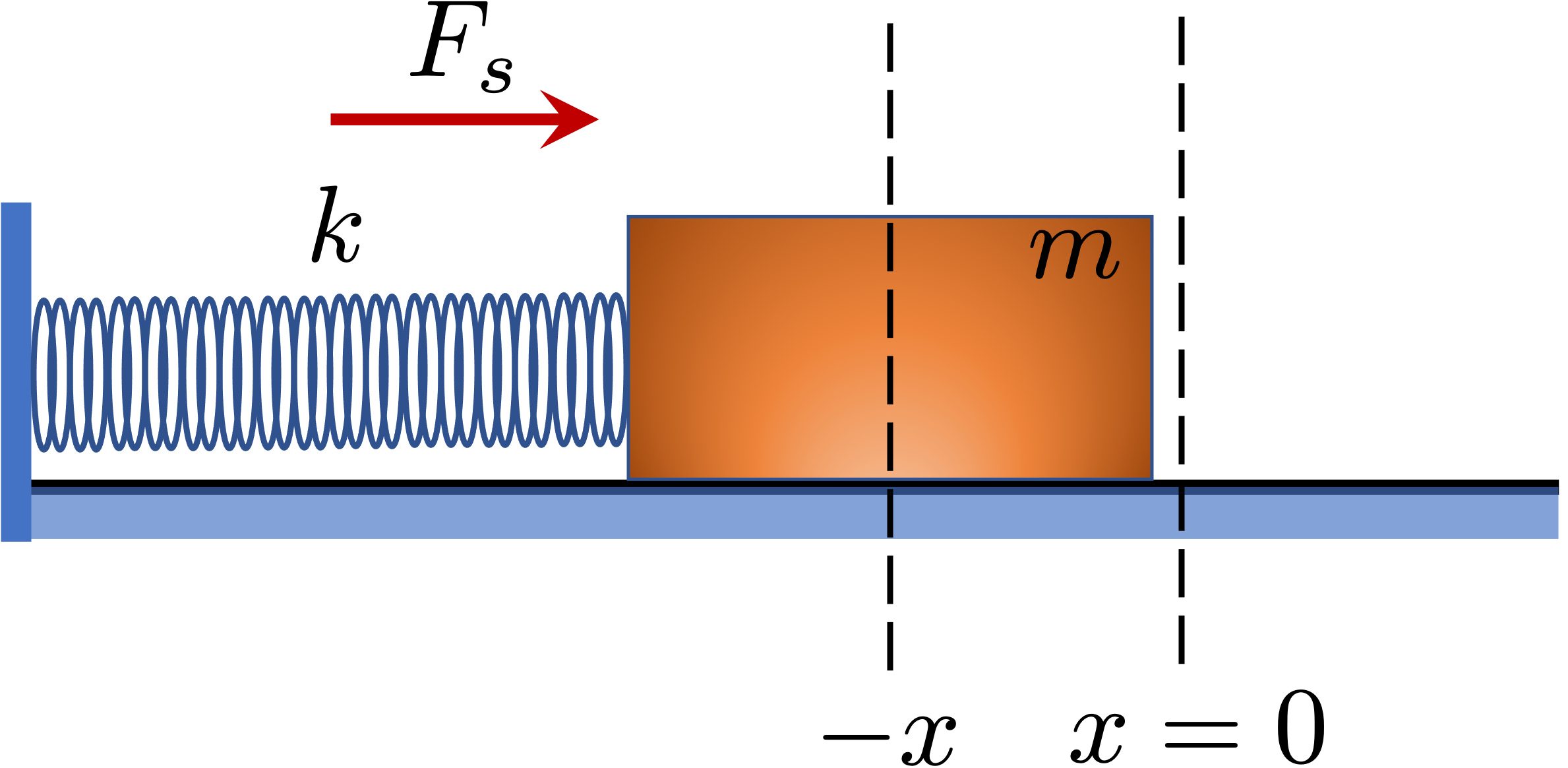
Consider an ideal spring which has the properties that it obeys Hooke's Law (see below) and is massless, as shown in Figure 1. A block of mass \(m\) is attached to the spring and the mass-spring system rests on the table with the spring at its equilibrium length. Consider compressing the spring by pushing on the mass, and the spring is compressed by a distance \(\Delta x\) as shown in Figure 2. Let us imagine that the there is no friction between the block and the surface of the table. You will notice that if you hold the system stationary at this position, then you will need to supply a force to prevent the spring from pushing the attached mass out. If the system is stationary as shown in Figure 2 then the force you supply will be exactly matched by the force that the spring exerts.

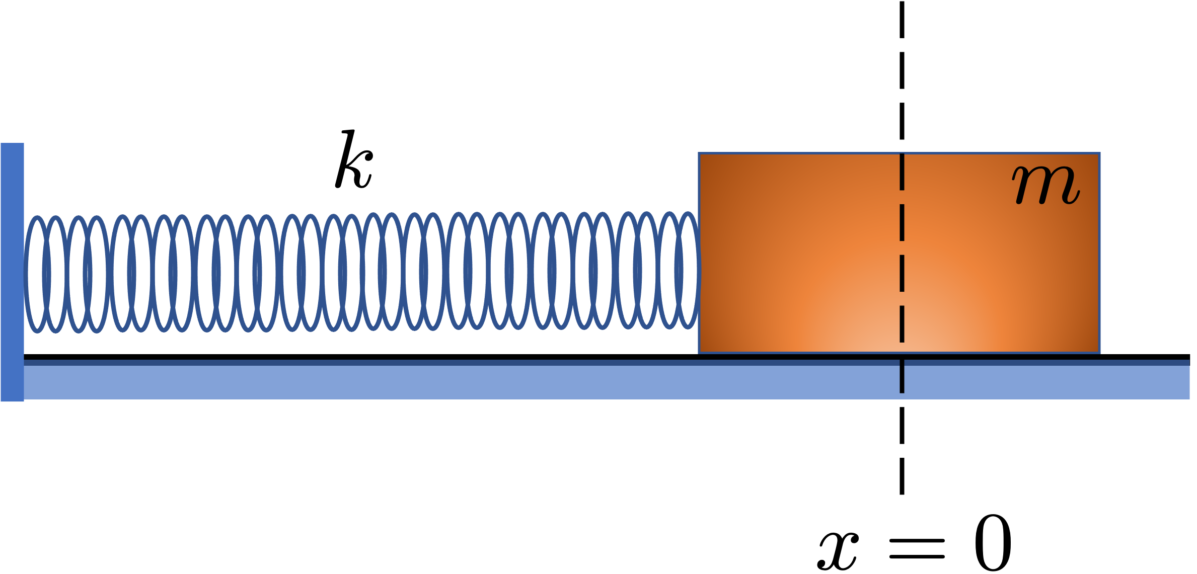
It also turns out that (for an ideal spring) the force that the spring exerts is proportional to the displacement of the spring away from its equilibrium length. Thus, this force can be written as,

\[ \vec{F}_s \propto \Delta \vec{x}. \label{eq:fsprop}\]

It turns out that the spring force is directed opposite to the displacement - hence you can see in Figure 2 the spring force is directed to the right when the displacement of the spring away from equilibrium is a vector pointing to the left. With this knowledge we can write Eq. \eqref{eq:fsprop} as an equality by inserting a constant of proportionality \(k\):

\[ \vec{F}_s = - k \Delta \vec{x}, \label{eq:hooke_s_law} \]

where \(k\) is called the spring constant. The stiffer the spring the larger the value of \(k\). Eq. \eqref{eq:hooke_s_law} is called Hooke's Law.

It can be readily seen that the relationship between the spring force and the displacement of the spring away from equilibrium is a linear relationship. You will be verifying this relationship in your lab today.

Conservation of Mechanical Energy

When you compressed the mass-spring system to the position shown in Figure 2 you did work on the system. Assuming that the system is stationary at this position, then the work that was done by you goes into increasing the potential energy of the mass-spring system. Now, the potential energy of the mass is unaltered, as it has not moved in the vertical direction, hence all the potential energy of the mass-spring system is given by the potential energy of the spring. Thus, when you did work to compress the spring, you transfered energy to the system and that energy is stored as potential energy in the compressed spring. The moment you let go of the mass, the system will move and it will convert this potential energy to kinetic energy of the mass.

When the system is dynamic, i.e., when the mass moves, in the absence of friction and other dissipative effects, the total mechanical energy of the system will remain conserved. In other words, for the mass-spring system the sum of the potential energy of the spring and the kinetic energy of the mass, at any given instant of time, will be constant. Therefore we can write,

\[ U + K = \textrm{const} \implies \frac{1}{2}kx^2 + \frac{1}{2}mv^2 = \textrm{const}. \label{eq:tot_energy} \]

Where we have used the definition of the potential energy stored in the spring, as well as the kinetic energy of the mass. In Eq. \eqref{eq:tot_energy} \(x\) represents displacement of the spring away from its equilibrium position, presumed to be \(0\), as shown in Figure 2. Therefore when \(v=0\) the kinetic energy is zero and the mass-spring system only has potential energy, and when the spring is at its equilibrium length, \(x=0\) and hence all of the energy of the system will be the kinetic energy of the mass. Thus, as the system moves energy will get converted from potential energy to kinetic energy and vice versa, however if you sum up the potential and kinetic energies at any given instant of time, you will find that the total mechanical energy is constant for the mass-spring system. You will be verifying Eq. \eqref{eq:tot_energy} in the lab today.

Work-kinetic energy theorem

Now consider the motion from the point of view of the block of mass \(m\) as shown in Figure 2. In the absence of friction and any dissipative effects the net force on the mass at any given instant is simply the spring force, and the latter is proportional to the displacement of the spring away from equilibrium. Hence we can immediately conclude that the net force on the mass is greatest in magnitude when the spring is displaced maximally from its equilibrium, and zero when the spring is momentarily at its equilibrium position during the ensuing motion of the mass-spring system. Therefore we can write that the change in kinetic energy of the mass must be equal to the work done on it by the net force, i.e., the spring force.

\[ W_\textrm{net} = \Delta K \implies \int_{x_1}^{x_2} \vec{F}_s \cdot \vec{dl} = K_2 - K_1, \label{eq:work_energy} \]

where, \(K_1\) and \(K_2\) are the kinetic energies of the mass at positions \(x_1\) and \(x_2\), respectively. You will be verifying Eq. \eqref{eq:work_energy} in the lab today.

If you would like to get a quick video refresher about a mass-spring system, see the following video.

Give it a go!

Data Analysis

Detemining the spring constant

After collecting the data be sure to export the data as csv files to your computer. You should have three separate csv files; the accelerometer, the force sensor and wheel sensor data.

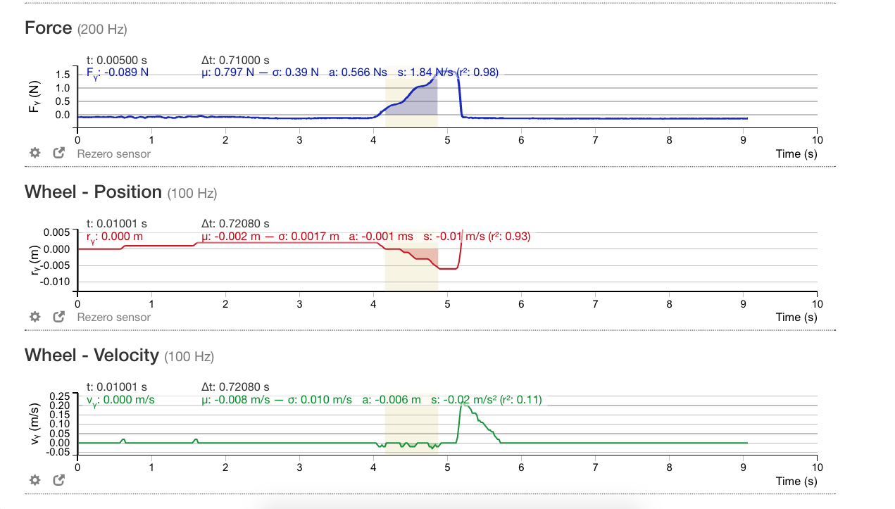
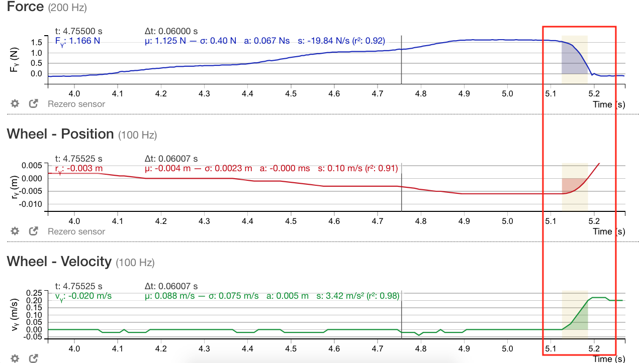
First, on the iOLab data collection software, zoom in on the force sensor, wheel position and wheel velocity data, as shown in Figure 3. Notice the highlighted portion of the data - this part of the data is when you are gently compressing the spring. Try to select a region where the force sensor data is linearly increasing. Try not to select the end-regions, but select an ample portion of the data in the middle of this increase, as shown in Figure 3. Carefully note down the beginning and end points of the time interval selected.

Next we will be working with the csv files to determine the spring constant. See the following video about how to carry out the analysis to determine the spring constant of the small spring.

Detemining the mass of the device

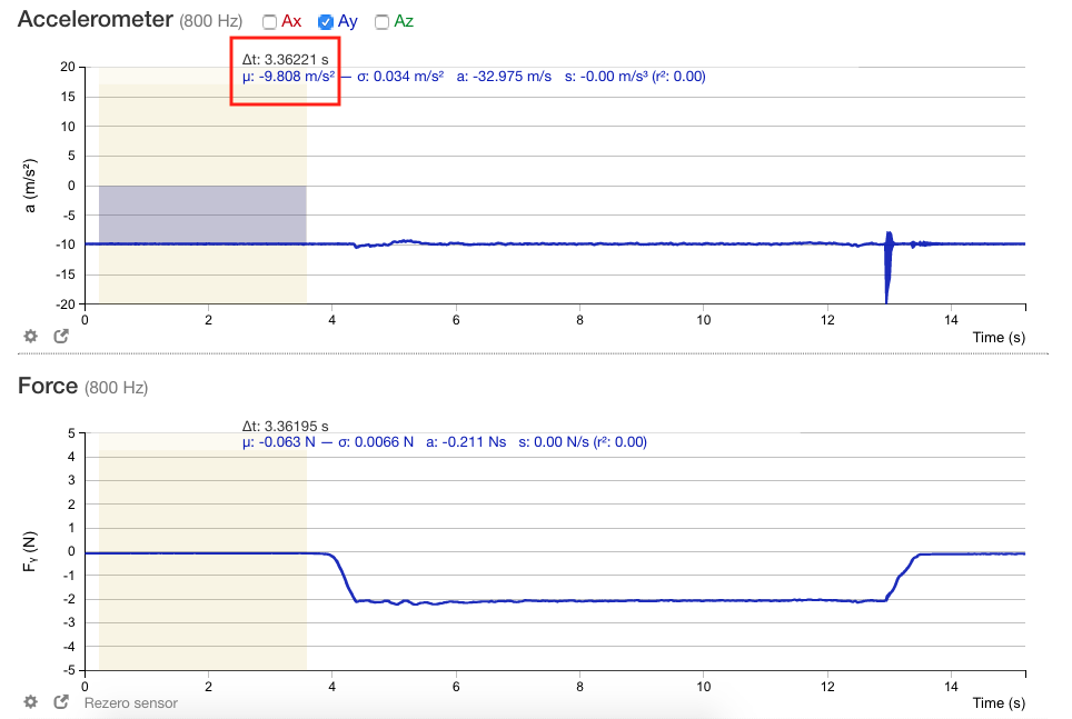
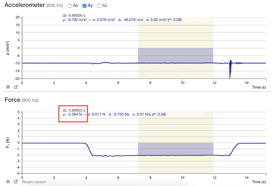
In the iOLab software open up the data you have collected in Part I for determining the mass of the iOLab device. First, determine the average value of the acceleration due to gravity when the device was resting on the table (see Figure 4 below). Carefully note down this average value of the acceleration. Next, determine the average value recorded by the force sensor when you lifted up the device; avoid the end regions of the interval, find the average somewhere in the middle of this region (see Figure 5 below). Carefully note down this average value of the force.. Divide the average force by the average acceleration to get the mass of the device. Carefully note down the value of the mass of the device you have determined.

Verifying Conservation of Mechanical Energy

In this part of the data analysis we will be looking at the portion of the data when the spring returns to equilibrium pushing the iOLab device forward. On the iOLab data collection software load the data from the experiment and select only the force sensor, the wheel position and the wheel velocity data. Once you have done so, carefully examine the force sensor data to identify the region where the spring returns to its natural length from its compressed state. This will be the portion of the data when the spring force decreases linearly. Zoom in on the three data sets so that it looks similar to the snapshot shown in Figure 6 below.

Carefully note down the initial and final wheel positions (\(x_1\) and \(x_2\)) and wheel velocities (\(v_1\) and \(v_2\)) of this interval. A CLUE FOR SELECTING THE INTERVAL PROPERLY: the initial wheel velocity should be \(v_1=0\), and the final wheel position of the interval should be \(x_2=0\) i.e., when the spring has returned to its equilibrium length.

Once you have noted down the values of \(x_1, x_2, v_1\) and \(v_2\), calculate the change in the potential energy of the spring, as well as the change in kinetic energy of the mass according to,

\[ \Delta U = \frac{1}{2}k(x_2^2-x_1^2) \label{eq:deltaU} \]

and

\[ \Delta K = \frac{1}{2}m(v_2^2-v_1^2). \label{eq:deltaK} \]

Where \(m\) is the mass of the device and \(k\) is the spring constant, as determined above. How do the values for the change in the potential energy and the change in the kinetic energy compare?

Verifying the Work-Kinetic Energy Theorem

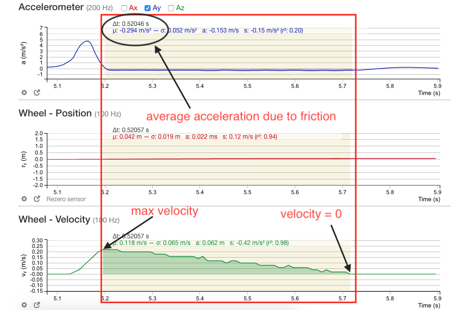
In this part of the data analysis you will be looking at the work done by friction on the iOLab device to slow it down to a dead stop. Open the iOLab data logging software and load the data from the run if it isn't already loaded. Select the accelerometer, wheel position and wheel velocity data. Apply a smoothing filter on the acceleration data, try not to use a smoothing filter higher than say "\(7\)" or "\(8\)". A smoothing filter of number \(n\) essentially averages the data around any point by considering \(n\) nearest neighbours around that point. Once you have smoothed the data zoom in on the part of the data when the iOLab device is in motion; i.e., it starts moving the moment you let it go and it stops moving a short time later as a result of friction dissipating energy from the system. The zoomed in data should look similar to that shown in Figure 7.

Note down the average value of the acceleration due to friction. Also note down the maximum velocity (\(v_m\)) of the iOLab device, i.e., the velocity of the iOLab device just as the spring reaches equilibrium length. The final velocity should be zero. You can determine the work done by friction, which is the net work done on the iOLab device according to

\[ W_{\textrm{net}} = m a_{_\textrm{avg}} d, \label{eq:wnet} \]

where \(m\) is the mass of the device and \(a_{_\textrm{avg}}\) is the average value of the acceleration due to friction determined above. \(d\) is the distance over which the friction acts; essentially the area under the Wheel-velocity graph as shown in Figure 7. Note that this work done should turn out to be negative as the acceleration is negative, i.e., a deceleration.

Next determine the change in the kinetic energy of the iOLab device. This is given by

\[ \Delta K = - \frac{1}{2} m v_m^2, \label{eq:delta_k2} \]

where again \(m\) is the mass of the device and \(v_m\) is the maximum velocity of the iOLab device as determined above. How does the net work done by friction compare with the change in kinetic energy of the device?